Gradient Descent

Learning Objectives

• Understand partial derivative and gradient

• Understand how gradient descent may be used in optimization problems

• Apply gradient descent in machine learning

Linear Approximation with Least Square Error

As mentioned in the previous section, supervised machinear learning can be formulated as a minimization problem: minimizing the error. This chapter starts with a problem that is probably farmiliar to many people already: linear approximation with least square error.

Consider a list of \(n\) points: \((x_1, \tilde{y_1})\), \((x_2, \tilde{y_2})\), …, \((x_n, \tilde{y_n})\). Please notice the convention: \(y = a x + b\) is the underlying equation and \(y\) is the “correct” value. It is generally not possible getting the correct value of \(y\) due to noise and limitation of meausrement instruments. Instead, we can get only the observed \(y\) with noise. To distinguish these two, we use \(\tilde{y}\) to express the observed value. It may be different from the true value of \(y\).

The problem is to find the values of \(a\) and \(b\) for a line \(y = a x + b\) such that

\(e(a, b)= \underset{i=1}{\overset{n}{\sum}} (y_i - (a x_i + b))^2\)

is as small as possible. This is the cumulative error. Let’s call it \(e(a, b)\) because it has two variables \(a\) and \(b\). Here we will solve this problem in two ways: analytically and numerically.

Analytics Method for Least Square Error

In Calculus, you have learned the concept of derivative. Suppose \(f(x)\) is a function of a single variable \(x\). The derivative of \(f(x)\) with respect to \(x\) is defined as

\(f'(x) = \frac{d}{dx} f(x) = \underset{h \rightarrow 0}{\text{lim}} \frac{f(x + h) - f(x)}{h}\)

The derivative calculates the ratio of change in \(f(x)\) and the change in \(x\). A geometric interpretation is the slope of \(f(x)\) at a specific point of \(x\).

Extend that concept to a multivariable function. Suppose \(f(x, y)\) is a function of two variables \(x\) and \(y\). The partial derivative of \(f(x,y)\) with respect to \(x\) at point \((x_0, y_0)\) is defined as

\(\frac{\partial f}{\partial x}| _{(x_0, y_0)} = \frac{d}{dx} f(x, y_0) | _{x = x_0} =\underset{h \rightarrow 0}{\text{lim}} \frac{f(x_0 + h, y_0) - f(x_0, y_0)}{h}\)

The derivative calculates the ratio of change in \(f(x, y)\) and the change in \(x\) while keeping the value of \(y\) unchanged.

Similarly, the partial derivative of \(f(x,y)\) with respect to \(y\) at point \((x_0, y_0)\) is defined as

\(\frac{\partial f}{\partial y}| _{(x_0, y_0)} = \frac{d}{dy} f(x_0, y) | _{y = y_0} =\underset{h \rightarrow 0}{\text{lim}} \frac{f(x_0, y_0 + h) - f(x_0, y_0)}{h}\)

To minimize the error function, we take the partial derivatives of \(a\) and \(b\) respectively:

\(\frac{\partial e}{\partial a} = 2 (a x_1 + b - y_1) x_1 + 2 (a x_2 + b - y_2) x_2 + ... + 2 (a x_n + b - y_n) x_n\)

\(\frac{\partial e}{\partial a} = 2 a (x_1^2 + x_2^2 + ... + x_n^2) + 2 b (x_1 + x_2 + ... + x_n) - 2 (x_1 y_1 + x_2 y_2 + ... + x_n y_n)\)

\(\frac{\partial e}{\partial a} = 2 (a \underset{i=1}{\overset{n}{\sum}} x_i^2 + b \underset{i=1}{\overset{n}{\sum}} x_i - \underset{i=1}{\overset{n}{\sum}} x_i y_i)\)

For \(b\):

\(\frac{\partial e}{\partial b} = 2 (a x_1 + b - y_1) + 2 (a x_2 + b - y_2) + ... + 2 (a \times x_n + b - y_n)\)

\(\frac{\partial e}{\partial b} = 2 a (x_1 + x_2 + ... + x_n) + 2 n b - 2 (y_1 + y_2 + ... + y_n)\)

\(\frac{\partial e}{\partial b} = 2 (a \underset{i=1}{\overset{n}{\sum}} x_i + b n - \underset{i=1}{\overset{n}{\sum}} y_i)\)

To find the minimum, set both to zero and obtain two linear equations of \(a\) and \(b\).

\(a \underset{i=1}{\overset{n}{\sum}} x_i^2 + b \underset{i=1}{\overset{n}{\sum}} x_i = \underset{i=1}{\overset{n}{\sum}} x_i y_i\)

\(a \underset{i=1}{\overset{n}{\sum}} x_i + b n = \underset{i=1}{\overset{n}{\sum}} y_i\)

The values of \(a\) and \(b\) can be expressed by

\(a =\frac{n \underset{i=1}{\overset{n}{\sum}} x_i y_i - \underset{i=1}{\overset{n}{\sum}} x_i \underset{i=1}{\overset{n}{\sum}} y_i}{n \underset{i=1}{\overset{n}{\sum}} x_i^2 - \underset{i=1}{\overset{n}{\sum}} x_i \underset{i=1}{\overset{n}{\sum}} x_i}\)

\(b =\frac{\underset{i=1}{\overset{n}{\sum}} y_i \underset{i=1}{\overset{n}{\sum}} x_i^2 - \underset{i=1}{\overset{n}{\sum}} x_i y_i \underset{i=1}{\overset{n}{\sum}} x_i}{n \underset{i=1}{\overset{n}{\sum}} x_i^2 - \underset{i=1}{\overset{n}{\sum}} x_i \underset{i=1}{\overset{n}{\sum}} x_i}\)

Let’s consider an example:

x	y
8.095698376	23.51683637
6.358470914	9.792790054
-9.053869996	-39.96474572
-8.718226575	-30.35310844
8.92002599	26.16662601
-9.304226583	-37.4223126
-4.413344816	-18.03547019
9.24473846	24.39367474
2.717746556	-4.589498946
5.87537092	15.7037148
-2.962047549	-7.508042385
-1.793005634	-11.81506333
-2.341379964	-14.96321124
4.742625547	2.282082477
-2.007598497	-5.068305913
9.333353675	28.44940642
2.570708237	3.086379154
-4.846225403	-25.6409577
2.571789981	7.795844519
-9.044770879	-26.25061389
5.09385439	8.166196092
-5.665252693	-21.99241714
1.193065754	0.698347441
-8.739601542	-31.96384225
-5.850434065	-17.51926158
4.556308579	9.854628779
-0.509866694	-10.85684654
-0.24261641	-8.33876201
7.930407455	19.56805947
6.201498841	5.836888055
-3.524341584	-19.45328039
6.034477356	19.15245129

The pairs are plotted below:

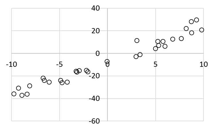
The value of \(y\) is calculated by

\(y = 3 x - 5 + \epsilon\)

here \(\epsilon\) is the error (or noise) and it is set to a randeom number between -8 and 8.

The figure shows the line without noise:

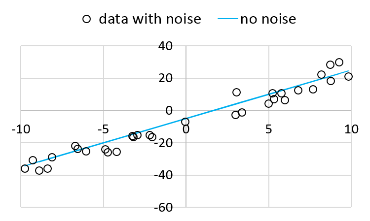
Using the equations, \(a = 3.11806\) and \(b = -5.18776\).

Next, we explain how to solve the problem using gradient descent.

Gradient

The gradient of a two-variable function \(f(x, y)\) is at point \((x_0, y_0)\) is defined as

\(\nabla f|_{(x_0, y_0)} = \frac{\partial f}{\partial x} {\bf i} + \frac{\partial f}{\partial y} {\bf j}\)

Here, \({\bf i}\) and \({\bf j}\) are the unit vector in the \(x\) and \(y\) directions.

Suppose \({\bf v} = \alpha {\bf i} + \beta {\bf j}\) is a unit vector. Then, the amount of \(f\)’s changes in the direction of \({\bf v}\) is the inner product of \(\nabla f\) and \({\bf v}\). The greatest change occurs at the direction when \({\bf v}\) is the unit vector of \(\nabla f\). Since \({\bf v}\) is a unit vector, if its direction is different from \(\nabla f\), the inner product must be smaller.

One way to understand graident is to think about speed bumps on roads.

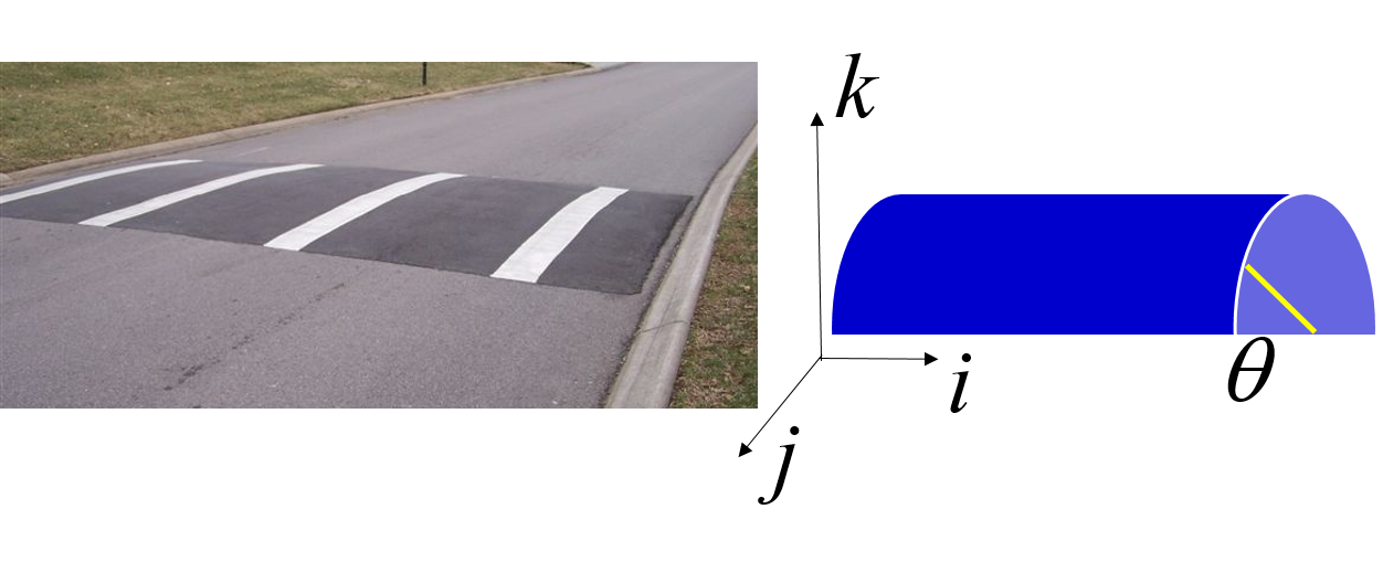
The bump is modeled as a half cylinder. For simplicity, we assume that the bump is infinitely long in the \(x\) direction. A point on the surface of the bump can be expressed as

\(p = x {\bf i} + \alpha \cos(\theta) {\bf j} + \beta \sin(\theta) {\bf k}\)

The gradient is

\(\nabla p = \frac{\partial p}{\partial x} {\bf i} + \frac{\partial p}{\partial y} {\bf j} + \frac{\partial p}{\partial z} {\bf k} = {\bf i} + \alpha (- \sin(\theta)) {\bf j} + \beta \cos(\theta) {\bf k}.\)

This is the tangent of the point on the surface.

Next, consider another vector (such as the tire of your unicycle) goes through this bump. We consider a unicycle because it is simpler: we need to consider only one wheel. What is the rate of changes along this surface? If you ride the unicycle along this bump without getting onto the bump, then the vector of your movement can be expressed by

\(v = x {\bf i}\)

How is this affected by the slope of the bump? The calculation is the inner product of the two vectors:

\(\nabla p \cdot v = x {\bf i}\).

Notice that this inner product contains no \(\theta\). What does this mean? It means that your movement is not affected by \(\theta\). This is obvious because you are not riding onto the bump.

Next, consider that you ride straight to the bump. The vector will be

\(v = - y {\bf j}\)

The slope of the bump affects your actual movement, again by the inner product:

\(\nabla p \cdot v = y \alpha \sin(\theta) {\bf j}\).

How can we interpret this? The moment when your tire hits the bump, \(\theta\) is zero so your tire’s movement along the \({\bf j}\) direction is zero. This is understandable because you cannot penetrate into the bump. When the tire is at the top of the bump, \(\theta\) is \(\frac{\pi}{2}\) and the tire has the highest speed.

Based on this understanding, it is easier to answer the following question: “Which direction along the surface gives the greatest changes?” Because the actual change is the inner product of the direction and the gradient, the greatest change occurs along the direction of the gradient.

Gradient Descent

Gradient Descent is a method for solving minimization problems. The gradient of a function at a point is the rate of changes at that point. Let’s consider a simple example: use gradient descent to find a line that has the smallest sum of square error. This is the same problem described above. The earlier solution uses formulae to find \(a\) and \(b\). Here, we will not use the formulae.

The gradient of a function is the direction of changes.

\(\nabla e = \frac{\partial e}{\partial a} {\bf i} + \frac{\partial e}{\partial b} {\bf j}\)

Suppose \(\Delta w = \alpha {\bf i} + \beta {\bf j}\) is a vector.

By definition, if \(\Delta w\) is small enough, then the change in \(\nabla e\) alogn the direction of \(\Delta w\) can be calculated as

\(\Delta e = \nabla e \cdot \Delta w\).

The goal is to reduce the error. Thus, \(\Delta w\) should be chosen to ensure that \(\Delta e\) is negative. If we make

\(\Delta w = - \eta \nabla e\),

then

\(\Delta e = \nabla e \cdot (- \eta \nabla e) = - \eta (\nabla e)^2\).

This ensures that the error \(e\) becomes smaller. The value \(\eta\) is called the learning rate. Its value is usually between 0.1 and 0.5. If \(\eta\) is too small, \(\Delta e\) changes very slowly, i.e., learning is slow. If \(\eta\) is too large, \(\Delta e = \nabla e \cdot \Delta w\) is not necessarily true.

Numerical Method for Least Square Error

It is possible to find an analytical solution for \(a\) and \(b\) because the function \(e\) is pretty simple. For many machine learning problems, the functions are highly complex and in many cases the functions are not even known in advance. For these problems, reducing the errors can be done numerically using data. This section is further divided into two different scenarios.

• The first assumes that we know the function \(e\) but we do not have formulaes for \(a\) or \(b\).

• The second assumes that we do not know the function \(e\) and certainly do not know the formulaes for \(a\) or \(b\). This is the common scenario.

For the first case,

\(\nabla e = \frac{\partial e}{\partial a} {\bf i} + \frac{\partial e}{\partial b} {\bf j}\)

\(\frac{\partial e}{\partial a} = 2 (a \underset{i=1}{\overset{n}{\sum}} x_i^2 + b \underset{i=1}{\overset{n}{\sum}} x_i - \underset{i=1}{\overset{n}{\sum}} x_i y_i)\)

\(\frac{\partial e}{\partial b} = 2 (a \underset{i=1}{\overset{n}{\sum}} x_i + b n - \underset{i=1}{\overset{n}{\sum}} y_i)\)

This is gradient1 below.

For the second case, the gradient can be estimated using the definition of partial derivative. This is shown in gradient2 below.

After finding the gradient using either method, the values of \(a\) and \(b\) change by \(- \eta \nabla e\).

#!/usr/bin/python3
# gradientdescent.py

import math
import random
import sys
import argparse

def readfile(file):
    # print(file)
    data = []
    try:
        fhd = open(file) # file handler
    except:
        return data
    for oneline in fhd:
        data.append(float(oneline))
    return data

def readfiles(f1, f2):
    x = readfile(f1)
    y = readfile(f2)
    return [x, y]

def sums(x, y):
    n = len(x)
    if (n != len(y)):
        print ("ERROR")
    sumx = 0
    sumx2 = 0
    sumy = 0
    sumxy = 0
    for ind in range(n):
        sumx = sumx + x[ind]
        sumy = sumy + y[ind]
        sumx2 = sumx2 + x[ind] * x[ind]
        sumxy = sumxy + x[ind] * y[ind]
    return [n, sumx, sumy, sumx2, sumxy]

def gradient1(a, b, n, sumx, sumy, sumx2, sumxy):
    pa = 2 * (a * sumx2 + b * sumx - sumxy)
    pb = 2 * (a * sumx + b * n - sumy)
    # convert to unit vector
    length = math.sqrt(pa * pa + pb * pb)
    ua = pa / length
    ub = pb / length
    return [ua, ub]

def gradient2(a, b, n, x, y):
    # use the definition
    # the partial derivative of function f respect to variable a is
    # (f(a + h) - f(a)) / h for small h
    h = 0.01
    error0 = 0
    errora = 0
    errorb = 0
    for ind in range(n):
        diff0 = y[ind] - (a * x[ind] + b)
        diffa = y[ind] - ((a + h) * x[ind] + b)
        diffb = y[ind] - (a * x[ind] + (b + h))
        error0 = error0 + diff0 * diff0
        errora = errora + diffa * diffa
        errorb = errorb + diffb * diffb
    pa = (errora - error0) / h
    pb = (errorb - error0) / h
    # convert to unit vector
    length = math.sqrt(pa * pa + pb * pb)
    ua = pa / length
    ub = pb / length
    return [ua, ub]

def findab(args):
    [x, y] = readfiles(args.file1, args.file2)
    '''
    method 1: know the formula for the gradient
    '''
    [n, sumx, sumy, sumx2, sumxy] = sums(x, y)
    # initial values for a and b
    a = -5
    b = 2
    eta = 0.1
    count =  1000
    while (count > 0):
        [pa, pb] = gradient1(a, b, n, sumx, sumy, sumx2, sumxy)
        a = a - eta * pa
        b = b - eta * pb
        count = count - 1
    print (a, b)
    '''
    method 2: do not know the formula
    '''
    a = -15
    b = 21
    count =  1000
    while (count > 0):
        [pa, pb] = gradient2(a, b, n, x, y)
        a = a - eta * pa
        b = b - eta * pb
        count = count - 1
    print (a, b)

def checkArgs(args = None):
  parser = argparse.ArgumentParser(description='parse arguments')
  parser.add_argument('-f1', '--file1', 
                      help = 'name of the first data file',
                      default = 'xval')
  parser.add_argument('-f2', '--file2', 
                      help = 'name of the second data file',
                      default = 'yval')
  pargs = parser.parse_args(args)
  return pargs


if __name__== "__main__":
  args = checkArgs(sys.argv[1:])
  findab(args)

The two methods get similar results: The first method gets 3.153 and -5.187 for \(a\) and \(b\) respectively. The second method gets 3.027 and -5.192.

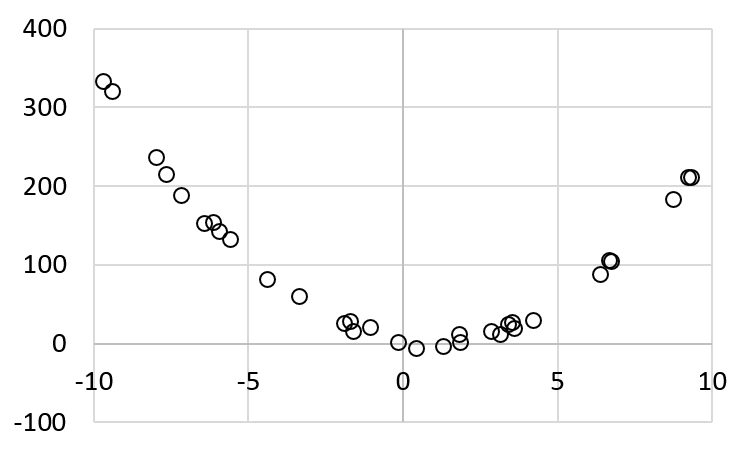
Numerical Method for Least Square Error of Quadratic Function

The examples above uses a linear function \(y = a x + b\). Now, let’s consider a more complex example: a quadratic function: \(y = a x^2 + b x + c\). The error function is defined by three terms: \(a\), \(b\), and \(c\).

\(e(a, b, c)= \underset{i=1}{\overset{n}{\sum}} (y_i - (a x_i ^ 2 + b x_i + c))^2\)

The value of \(y\) is calculated by

\(y = 3 x^2 - 5 x + 4 + \epsilon\)

here \(\epsilon\) is the error (or noise) and it is set to a randeom number between -8 and 8.

x	y
-3.370103805	60.79185325
0.417414305	-5.323619187
-6.159102555	154.3634865
-4.407403766	82.5948879
9.217171131	211.5745285
-7.174813026	188.278774
6.361795959	88.5112383
1.79223335	11.99774387
-1.926842791	26.55005374
3.11961916	12.0001045
3.407105822	25.23458989
3.516276644	27.86258459
-6.446048868	153.4091251
-1.611122918	16.29112594
-9.423197392	320.9271831
-0.163191843	1.413342642
-7.984372477	237.3069972
-1.083286108	20.77621844
-1.721374317	28.35361787
9.307151676	211.0397578
2.847589125	15.49036578
-9.704318719	333.9723539
6.652947501	106.6501811
1.286261333	-2.972412887
6.730248976	104.7116952
4.198544935	29.78821666
8.730545018	183.571542
-5.944582098	142.8709084
3.596351215	19.40151
-5.606758376	132.9978749
-7.680210557	215.0928846
1.852911853	2.423800574

The pairs are plotted below:

The program for calculating \(a\), \(b\), and \(c\) needs only slight changes from the previous program:

#!/usr/bin/python3
# gradientdescent2.py

import math
import random
import sys
import argparse

def readfile(file):
    # print(file)
    data = []
    try:
        fhd = open(file) # file handler
    except:
        return data
    for oneline in fhd:
        data.append(float(oneline))
    return data

def readfiles(f1, f2):
    x = readfile(f1)
    y = readfile(f2)
    return [x, y]

def quadraticvalue(a, b, c, x):
    val = a * x * x + b * x + c
    return val

def gradient(a, b, c, n, x, y):
    # use the definition
    # the partial derivative of function f respect to variable a is
    # (f(a + h) - f(a)) / h for small h
    # h = random.random() * 0.5 # make it small
    h = 0.01
    error0 = 0
    errora = 0
    errorb = 0
    errorc = 0
    for ind in range(n):
        diff0 = y[ind] - quadraticvalue(a, b, c, x[ind])
        diffa = y[ind] - quadraticvalue(a + h, b, c, x[ind])
        diffb = y[ind] - quadraticvalue(a, b + h, c, x[ind])
        diffc = y[ind] - quadraticvalue(a, b, c + h, x[ind])
        error0 = error0 + diff0 * diff0
        errora = errora + diffa * diffa
        errorb = errorb + diffb * diffb
        errorc = errorc + diffc * diffc
    pa = (errora - error0) / h
    pb = (errorb - error0) / h
    pc = (errorc - error0) / h
    # convert to unit vector
    length = math.sqrt(pa * pa + pb * pb + pc * pc)
    ua = pa / length
    ub = pb / length
    uc = pc / length
    return [ua, ub, uc]

def findabc(args):
    [x, y] = readfiles(args.file1, args.file2)
    '''
    do not know the formula
    '''
    a = random.randint(-10, 10)
    b = random.randint(-10, 10)
    c = random.randint(-10, 10)
    count =  10000
    n = len(x)
    eta = 0.1
    while (count > 0):
        [pa, pb, pc] = gradient(a, b, c, n, x, y)
        a = a - eta * pa
        b = b - eta * pb
        c = c - eta * pc
        count = count - 1
    print (a, b, c)

def checkArgs(args = None):
  parser = argparse.ArgumentParser(description='parse arguments')
  parser.add_argument('-f1', '--file1', 
                      help = 'name of the first data file',
                      default = 'xval2')
  parser.add_argument('-f2', '--file2', 
                      help = 'name of the second data file',
                      default = 'yval2')
  pargs = parser.parse_args(args)
  return pargs


if __name__== "__main__":
  args = checkArgs(sys.argv[1:])
  findabc(args)

Running this program ten times gets the following results:

a	b	c
3.011255896382324	-5.237109053403006	4.587766159787751
2.9118463569721067	-5.235739889402345	4.558316574435434
2.913418168901663	-5.236030395939285	4.611313910795599
3.01028934524673 9	-5.237423283136554	4.6514776776523155
3.0116767376997156	-5.2370171800113	4.568807336762989
3.0116145023680554	-5.237035419533481	4.572520167800626
2.911538900320818	-5.2359055455148615	4.591420135857997
2.908676740232057	-5.2363349865534214	4.682182248171528
2.911471635130624	-5.235840824838787	4.5789355660578455
2.911385934228692	-5.235874673892769	4.585754511975301

The calculated values are pretty consistent.

Gradient Descent for Neural Networks

Three-Layer Neural Networks

Neural networks are the foundation of the recent impressive progress in machine learning. The problems described so far have pretty clear mathematical foundations (for example, linear approximation or quadratic approximation). More complex problems can be difficult to express mathematically. Let’s consider an example in our everyday life: How do you describe a “chair”? “Simple”, you may say. You define “A chair has four legs with a flat surface on which a person can sit, like this figure”:

If that is a chair, how about this one? “Well, that is also a chair.”, you may say.

You change your answer to “A chair has two or four legs with a flat surface on which a person can sit.” There are still problems: How about the following two? Are they chairs?

As you can see, it is not so easy to define a chair.

The same problem occurs in many other cases. How do you define a car? You may say, “A car is a vehicle with four wheels and can transport people.” Some cars have only three wheels. Some cars have six wheels. Some cars do not transport people.

Instead of giving a definition, another approach is to give many examples and a complex enough function so that the function can learn the common characteristics of these examples. Neural networks are complex non-linear functions and they have the capabilities of learning from many examples. More details about neural networks will be covered in later chapters. This chapter gives only a few simple examples showing how gradient descent can be used to learn.

Neural networks use one particular architecture for computing. This architecture is inspired by animal brains where billions of neurons are connected. This book does not intend to explain how neural networks resemble brains, nor the biological experiments discovering the mechanisms of brain functions. Instead, this section solve relatively simple problems (creating logic gates) using this particular architecture.

The following figure is an example of a neural network with three layers: an input layer, an output layer, and a hidden layer. A layer is hidden simply because it is neither the input layer nor the output layer.

Figure 65 Neural network of three layers

In this example, the input layer has two neurons (neurons 0-1), the hidden layer has four neurons (neurons 0-3), and the output layer has two neurons (neurons 0-1). Prior studies show that a neural network with only two layers (input and output) without any hidden layer has limited capability. Thus, almost all neural networks have hidden layers. Some complex networks can have dozens or even hundreds of hidden layers. It has been shown that deep neural networks can be effective learning complex tasks. Here, deep means neural networks have many hidden layers. Information moves from the layers on the left toward the layers on the right. There is no feedback of information. Nor do two neurons of the same layer exchange information. Different layers may have different numbers of neurons.

Figure 66 Connects neurons of different layers. These are the only connections between enurons. Please notice that the numbers of neurons are 2, 4, and 2 in the three layers.

The neurons in two adjacent layers are connected by weights, are expressed as a three-dimensional array:

\(weights[l][s][d]\)

connects the neuron at layer \(l\) to layer \(l + 1\); \(s\) is the source and \(d\) is the destination. It is also written as \(w_{l, s, d}\). Please notice that the indexes start from zero.

Figure 67 Definition of the indexes for weights

In the example, the left weight \(weights[0][1][2]\) has the first index 0 because it connects the input layer (layer 0) with the hidden layer (layer 1). From the top, this is the second neuron of the input layer; thus, the second index is 1. The destination is the third neuron in the hidden layer and the index is 2. The right weight is \(weights[1][3][0]\). The first index is 1 because it is from the hidden layer (layer 1). The second index is 3 because the source is the fourth neuron from the top. The destination is the first neuron in the output layer; thus, the third index is 0.

Each neuron performs relatively simple calculation, as shown below.

Figure 68 Computation performed by one neuron

A neuron in the input layer has only one input (only \(x_i\)) and the weight is always 1. A neuron in the hidden or the output layer has multiple inputs. Each neuron performs three stages of computation. First, the products of the input and the weight are added.

\(\underset{k = 0}{\overset{n-1}{\Sigma}} x_k w_k\).

Next, a constant called bias is added

\(b + \underset{k = 0}{\overset{n-1}{\Sigma}} x_k w_k\).

The value is then passed to an activation function \(f\). This must be a non-linear function because linear functions are too limited in their ability to handle complex situations.

Note

The world is not linear. Imagine that you really love chocolate. If you eat one piece of chocolate, you feel pretty good. If you eat two pieces of chocolate, you feel even better. Does this mean you feel better and better after you eat more and more chocolate? No. After you eat a lof of chocolate, you may feel that’s enough and want to stop. The same situation applies to everything. Imagine you get paid $20 an hour. If you work for two hours, you get $40. Can you make more and more money if you work longer and longer? No. First, each day has only 24 hours. You can make at most $480 per day if you do not sleep. If you do not sleep, you will fall ill soon and have to stop working.

Several activation functions are popular. This section uses the sigmoid function, expressed as \(\sigma(x)\), is one of the most widely used:

\(\sigma(x) = \frac{1}{1 + e^{-x}}\).

Because \(e^{-x} > 0\), \(\sigma(x)\) is always between 0 and 1.

The \(\sigma\) function has a special property: the derivative of \(\sigma(x)\) can be calculated easily:

\begin{eqnarray} & \frac{d \sigma(x)}{d x} \\ & = \frac{d}{dx} (\frac{1}{1 + e^{-x}}) \\ & = - \frac{1}{(1 + e^{-x})^2} \frac{d}{dx} (1 + e^{-x}) \\ & = \frac{e^{-x}}{(1 + e^{-x})^2} \\ & = \frac{1}{1 + e^{-x}} \frac{e^{-x}}{1 + e^{-x}} \\ & = \frac{1}{1 + e^{-x}} \frac{1 + e^{-x} - 1}{1 + e^{-x}} \\ & = \sigma(x) (1 - \sigma(x)). \end{eqnarray}

What does this mean? It means that we can calculate \(\frac{d \sigma(x)}{d x}\) if we know \(\sigma(x)\) without knowing the value of \(x\). If the value of \(\sigma(x)\) is \(v\) for a particular value of \(x\), then the derivative of is \(v (1-v)\).

Consider the following neuron. It has two inputs with values 0.99 and 0.01 respectively. The weights are 0.8 and 0.2. The bias is 0.3.

Figure 69 Example to calculate a neuron’s output

The value of \(s\) is 0.3 + 0.99 \(\times\) 0.8 + 0.01 \(\times\) 0.2 = 1.094. After the sigmoid function, this neuron’s output is

\(\frac{1}{1+ e^{-1.094}} = 0.7491342\).

Next, consider a complete neural network with all weights and biases:

Figure 70 Example to calculate a neural network’s outputs

The following table shows how to calculate the outputs of the four neurons in the hidden layer:

neuron	input	weight	bias	sum	output
0	0.99	0.7	0.1	0.798	0.689546499265968
	0.01	0.5
1	0.99	0.8	0.3	1.094	0.749134199078648
	0.01	0.2
2	0.99	0.8	0.5	1.2955	0.785076666300568
	0.01	0.35
3	0.99	0.6	0.4	0.9965	0.730369880613158
	0.01	0.25

How are these numbers calculated. This is the procedure for the first neuron:

\(s = 0.1 + 0.99 \times 0.7 + 0.01 \times 0.5 = 0.798\)

\(\frac{1}{1 + e^{-0.798}} = 0.689546499265968\)

The next table shows how the outputs are calculated.

neuron	input	weight	bias	sum	output
0	0.689546499265968	0.33	0.27	1.5473332709399	0.824528239528756
	0.7491341990786481	0.16
	0.785076666300568	0.31
	0.730369880613158	0.94
1	0.689546499265968	0.28	0.45	1.75723688345954	0.852863261520065
	0.7491341990786481	0.76
	0.785076666300568	0.48
	0.730369880613158	0.23

The outputs of the two neurons are 0.824528239528756 and 0.852863261520065.

Gradient Descent in Neural Networks (Backpropagation)

How can the concept of gradient descent be used to make neural networks produce the desired outputs? The answer is to adjust the weights and the biases. More precisely, the adjustment starts from the outputs toward the inputs and it is called back propagation. For the three layer networks shown above, the changes start from \(weight[1]\) based on the differences of the desired and the actual outputs. After adjusting \(weight[1]\), the method adjusts \(weight[0]\) between the hidden layer and the input layer.

When the actual outputs are different from the expected outputs, the difference is called the error, usually expressed as \(E\). Consider the following definition of error:

\(E = \underset{k=0}{\overset{t-1}{\sum}} \frac{1}{2} (exv_k - aco_k)^2\),

Here \(exv_k\) is the expect value and \(aco_k\) is the actual output of the \(k^{th}\) neuron (among \(t\) neurons). This definition adds the squares of errors from all output neurons. Do not worry about the constant \(\frac{1}{2}\) because it is for convenience here. It will be cancelled later.

Gradient descent can also be used to reduce the errors. The process is more complex than the previous examples because neural networks are more complex: We can change the weights but their effects go through the non-linear activiation function. It is not easy expressing the relationships between the error and the weights. In other words, the effects of weights go through a composition of functions (additions first and then the non-linear function).

Chain Rule

Before explaining how to adjust the weights, let’s review function composition. Consider that \(f(x)\) and \(g(x)\) are functions. We can create a composition of these two functions. For example, suppose \(f(x) = 3 x + 8\) and \(g(x) = (x + 1) ^ 2\). The composition of \(f(x)\) and \(g(x)\) can be written as:

\((f \circ g)(x) = f(g(x)) = f((x+1)^2) = 3 (x + 1) ^ 2 + 8 = 3 x^2 + 6 x + 11\).

In this case, \(g(x)\) is applied first and then \(f(x)\).

It is also possible to switch the order of the composition, written differently:

\((g \circ f)(x) = g(f(x)) = g(3x + 8) = ((3x + 8) + 1) ^ 2 = 9 x^2 + 54 x + 81\).

In this case, \(f(x)\) is applied first and then \(g(x)\).

What happens if we want to calculate the effect of changes in \(x\) to the composite function \((f \circ g)(x)\)? We need to apply the chain rule.

\((f \circ g)'(x) = f'(g(x)) \cdot g'(x)\).

Let’s validate this by using the example:

\((f \circ g)(x) = 3 x ^ 2 + 6 x + 11\).

Thus, \((f \circ g)'(x) = 6 x + 6\).

Next, we calculate \(f'(x) = 3\) and \(g'(x) = 2 x + 2\).

\((f \circ g)'(x) = f'(g(x)) \cdot g'(x) = 3 (2 x + 2) = 6x + 6\).

Error and Weights between Output and Hidden Layers

Figure 71 Definitions of the symbols

Symbols and their meanings:

symbol	meaning
\(r\)	number of neurons in the input layer
\(s\)	number of neurons in the hidden layer
\(t\)	number of neurons in the output layer
\(i\)	index of a neuron in the input layer \(0 \le i < r\)
\(j\)	index of a neuron in the hidden layer \(0 \le j < s\)
\(k\)	index of a neuron in the output layer \(0 \le k < t\)
\(\beta_j\)	bias of the \(j^{th}\) neuron in the hidden layer
\(b_k\)	bias of the \(k^{th}\) neuron in the output layer
\(u_i\)	input to the \(i^{th}\) neuron in the input layer
\(x_j\)	input to the \(j^{th}\) neuron in the hidden layer
\(y_j\)	output of the \(j^{th}\) neuron in the hidden layer
\(z_k\)	input to the \(k^{th}\) neuron in the output layer
\(aco_k\)	output of the \(k^{th}\) neuron in the output layer
\(exv_k\)	expected value of the \(k^{th}\) neuron in the output layer
\(\psi_{i,j}\)	weight connecting the \(i^{th}\) and \(j^{th}\) neurons
\(w_{j, k}\)	weight connecting the \(j^{th}\) and \(k^{th}\) neurons
\(\eta\)	learning rate

Here are the equations expressing the relationships among these terms:

Error: \(E = \underset{k=0}{\overset{t-1}{\sum}} \frac{1}{2} (aco_k - exv_k)^2\),

Actual output of the \(k^{th}\) neuron: \(aco_k = \sigma(z_k)\)

Input to the \(k^{th}\) neuron: \(z_k = b_k + \underset{j=0}{\overset{s-1}{\sum}} y_j w_{j,k}\)

Output of the \(j^{th}\) neuron: \(y_j = \sigma(x_j)\)

Input to the \(j^{th}\) neuron: \(x_j = \beta_j + \underset{i=0}{\overset{r-1}{\sum}} u_i \psi_{i,j}\)

Now, we can apply the chain rule to calculate the relationship between the error and a weight or a bias. Consider the output of a particular neuron. The expected value is a constant and its derivative is zero. Thus, we can ignore \(\frac{\partial exv_k}{\partial w_{j,k}}\). Instead, we need to worry about only the relationship between the actual output \(aco_k\) and a weight \(w_{j,k}\).

\(\frac{\partial E}{\partial w_{j,k}} = \frac{\partial E}{\partial aco_k} \frac{\partial aco_k}{\partial w_{j,k}}\)

\(\frac{\partial E}{\partial aco_k} = (aco_k - exv_k)\), because \(aco_k\) does not depend on any other neuron in the output layer.

As you can see, the constant \(\frac{1}{2}\) has been cancelled.

Applying the chain rule again:

\(\frac{\partial aco_k}{\partial w_{j,k}} = \frac{\partial aco_k}{\partial z_k} \frac{\partial z_k}{\partial w_{j,k}}\).

As explained earlier, \(\frac{\partial aco_k}{\partial z_k} = \sigma(z_k)(1 - \sigma(z_k)) = aco _k(1 - aco_k)\).

\(\frac{\partial z_k}{\partial w_{j,k}} = y_j\).

Now, we can put everything together:

\(\frac{\partial E}{\partial w_{j,k}} = (aco_k - exv_k) aco_k (1 - aco_k) y_j\).

Using gradient descent, we want to change the weight

\(\Delta w_{j,k} = - \eta \frac{\partial E}{\partial w_{j,k}} = - \eta (aco_k - exv_k) aco_k (1 - aco_k) y_j\).

Similarly,

\(\frac{\partial E}{\partial b_k} = (aco_k - exv_k) aco_k (1 - aco_k)\).

To change the bias:

\(\Delta b_k = - \eta \frac{\partial E}{\partial b_k} = - \eta (aco_k - exv_k) aco_k (1 - aco_k)\).

Error and Weights between Hidden and Input Layers

Next, we adjust the weights between the input and the hidden layer. The problem of the hidden layer is that we do not have expected values for the neurons. Instead, we must rely on the expected values at the output layer. This is called back propagation: propagating the expected values from the output layer to the hidden layer in order to adjust the weights. Consider the weight \(\psi_{i,j}\) between the \(i^{th}\) neuron of the input layer and the \(j^{th}\) neuron in the hidden layer. This weight may affect every neuron in the output layer.

Continue from the previous derivation, the output of the neuron \(y_j\) depends on the values of the input layer, the weights between the input layer and the hidden layer, and the bias. To avoid confusion, here \(\psi\), instead of \(w\), is used to express the weight between the input and the hidden layer.

How does the weight \(\psi_{i,j}\) affects the error? We can apply the chain rule again:

\(\frac{\partial E}{\partial \psi_{i,j}} = \frac{\partial }{\partial \psi_{i,j}} \underset{k=0}{\overset{t-1}{\sum}} \frac{1}{2} (aco_k - exv_k)^2 = \underset{k=0}{\overset{t-1}{\sum}} (aco_k - exv_k) \frac{\partial aco_k}{\partial \psi_{i,j}}\)

Our next step is to calculate \(\frac{\partial aco_k}{\partial \psi_{i,j}}\)

We can apply the chair rule again:

\(\frac{\partial aco_k}{\partial \psi_{i,j}} = \frac{\partial aco_k}{\partial z_k} \frac{\partial z_k}{\partial \psi_{i,j}} = aco_k (1 - aco_k) \frac{\partial z_k}{\partial \psi_{i,j}}\)

\(\frac{\partial z_k}{\partial \psi_{i,j}} = \frac{\partial z_k}{\partial y_j} \frac{\partial y_j}{\partial \psi_{i,j}} = w_{j, k} \frac{\partial y_j}{\partial \psi_{i,j}}\)

Apply the chain rule and we can get

\(\frac{\partial y_j}{\partial \psi_{i,j}} = \frac{\partial y_j}{\partial x_j} \frac{\partial x_j}{\partial \psi_{i,j}} = y_j (1 - y_j) \frac{\partial x_j}{\partial \psi_{i,j}}\)

Finally, \(\frac{\partial x_j}{\partial \psi_{i,j}} = u_i\).

Put everything together:

\(\frac{\partial E}{\partial \psi_{i,j}} = \underset{k=0}{\overset{t-1}{\sum}} (aco_k - exv_k) aco_k (1 - aco_k) w_{j, k} y_j (1 - y_j) u_i\)

Using gradient descent, we want to change the weight

\(\Delta \psi_{i,j} = -\eta \underset{k=0}{\overset{t-1}{\sum}} (aco_k - exv_k) aco_k (1 - aco_k) w_{j, k} y_j (1 - y_j) u_i\)

Similarly,

\(\Delta \beta_j = -\eta \underset{k=0}{\overset{t-1}{\sum}} (aco_k - exv_k) aco_k (1 - aco_k) w_{j, k} y_j (1 - y_j)\).

Neural Networks as Logic Gates

After understanding the operations of neural networks, it is time to use neural networks doing something useful. This example considers building a two-input logic gate. Each gate receives either false (also represented by 0) or true (also represented by 1). Commonly used gates are shown in the table below:

input 0	input 1	AND	OR	XOR
0	0	0	0	0
0	1	0	1	1
1	0	0	1	1
1	1	1	1	0

Prior studies have shown that it would not be possible make an XOR gate without any hidden layer. We won’t talk about that here. Instead, right now we focus on how to use graident descent to create logic gates.